Some words

‘R’ is a complete, flexible and open source system for statistical analysis which has become a core tool of choice for a wide range of researchers spanning over multiple disciplines. The aim of the present workshop is to give participants a first step hands-on practical session on the ‘R’ environment by introducing the basic principles and most used commands to help them explore and visualize their data.

What is R?

R is an open source complete and flexible software environment for statistical computing and graphics.

It includes:

Facilities for data import, storage in memory and manipulation
Functions for calculations on vectors and matrices
Large set of data analysis tools
Graphical tools
As a programming language, a simple development environment, with a text editor
R itself is written primarily in C and Fortran, and is an implementation of the statistical language S.

Advantages

Availability and compatibility
- R is free and is documented (manuals, reference sheets, mailing lists, blogs, and a wiki)
- Can run on all major operating systems and code is often portable too
State-of-the-art graphics capabilities
- R can produce quality graphical output in all of the standard formats (PDF, PS, EPS, JPEG, PNG, TIFF,…)
Can import files from other statistical programs
- Such as Minitab, S, SAS, SPSS, or Stata (NOT from GraphPad Prism)
- Other file types such as tab-delimited text (tsv), comma-separated values (csv), and even Excel (xls) with proper packages
Learn to program and do reproducible research
- It allows users to learn the basics of computer programming
- Writing scripts allows users to have a permanent, repeatable, annotated, cross-platform, shareable record of their analysis
- Automatic report generation that contain the code and the output of R scripts in various format (knitr and rmarkdown packages)
Speak the common language
- Knowing the basics of a tool will enhance the communication between collaborators and help in sharing information and data more easily
- R skills are in very high demand

Drawbacks

“Expert friendly”
- It is not very easy to learn and it takes time (steep learning curve)
- Needs prior formatting of the data
(Too) large amount of resources
- Lots of documentation and manuals available, might be cryptic
- Sometimes easy to get lost
Constantly evolving
- Can lead to backward-compatibility issues
Memory intensive and slow at times

R-studio environment

Launch it and let’s have a look

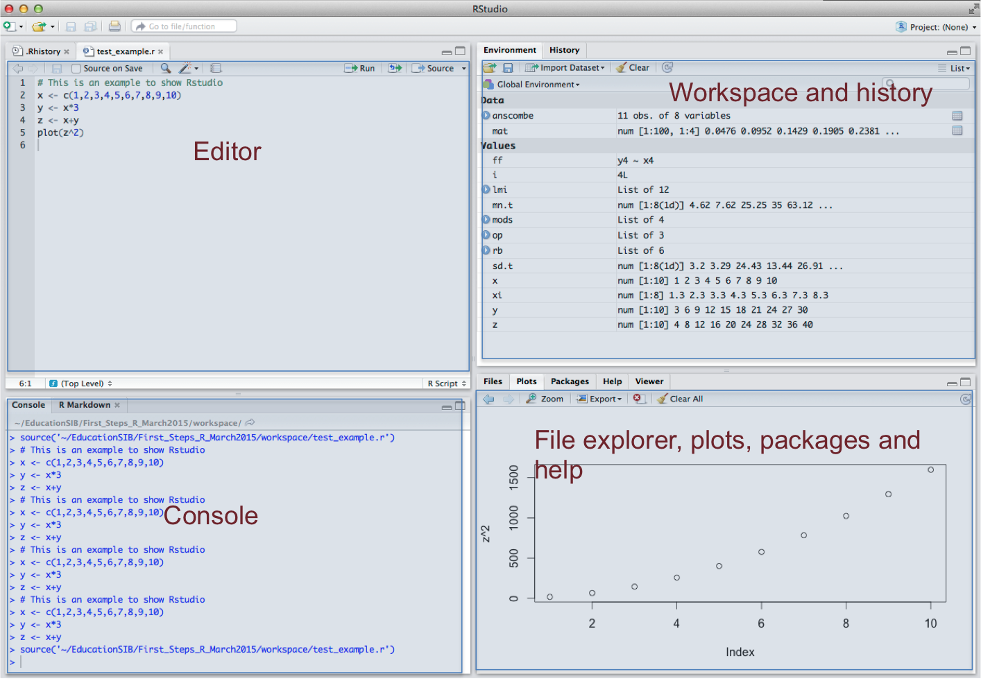
r-studio-env

Some environmental Functions

help() or ?—> To ask for help !!!
getwd() —> to print out the directory that is considered as working directory
setwd("path_to/the_directory/I_would_like_to/work_in") —> To set the directory that we would like it to be used as working directory
save.history() and load.history() —> The commands History so everything typed as commands will be remembered
save.image() and load.image() —> The environment will be saved not only the commands but also their output and all data loaded (size could become significantly big)
Create an R script: from the upper menu select File-->New File-->R Script, you can name it and choose the location Note To set your working directory without typing code, you can select from the upper menu Session-->Set Working Directory-->Choose Directory...
To execute a command from your R script, select the line or lines you want to execute and use the bottom located on the upper right corner of your script
To comment a script with explanatory sentences you don’t want to execute you simply need to add the # just before the sentence

Let’s warm up, ready!!!
On your own operating systems:

Create a directory on your computers and name it R-course
Download the course materials provided on site or by email and put it in R-course directory you have just created

In R-studio:

Create an R script and name it, save it in R-course directory
Set your working directory to R-course by command line or by using the R-studio menu

setwd("/The/location/of/my/R-course.R")

Check what is your current working directory by typing the command in the R-script you have just created (From now on you will be typing commands in this area)

getwd()

Comment your script (at the top to start with)

# This a comment on top of my command 
getwd()
getwd() # I can also comment my code at the level of my command

Generalities

Calculator

4 + 2
4 - 2 
4 * 2
4 / 2
4 ^ 2
sqrt(4)

Assigning variables

a <-1
b <- "I am learning R - it looks cool !!"
b

Q0- Assign the following “Hello everyone!” to a variable and call the variable on the next line

He<-"Hello everyone"
He

Functions

v<-c(2,4,5) # the vector function c()
# We can also use functions over functions
mean(v)

Printing output

print("Hello World")

Data Types

Use the function class() to determine the data type of the following (N.B. assign every number to a variable before calling class() function):

a<-7.5
class(a)

b<-7
class(b)

“whatever”

c<-"whatever"
class(c)

b+2i

d<-b+2i
class(d)

e<-b>a
class(e)

There are several logical operators &, |, ! among others.

f<-TRUE
g<-FALSE

Q1- Run the two lines above and Try those operators on f and g and comment

f<-TRUE
g<-FALSE
f&g
f|g
!f
!g

Vectors

Integers c(1,3,5)
Booleans c(FALSE, TRUE, FALSE, TRUE)
String c("I","am","in","a","good","mood")

Q2- We could you use functions over vectors, for example: try the function length() over the string vector above

length(c("I","am","in","a","good","mood"))

Look at the following code:
functions as.factor(), levels() and nlevels()

v0<-c("I","am","in","a","good","mood","I","am","in","a","good","mood")
levels(as.factor(v0))
nlevels(as.factor(v0))

Integers v1<-c(1,3,5) String v2<-c("I","am","in","a","good","mood")

Q3- Use the function c() to merge vector v1 and v2

What do you notice?

v1<-c(1,3,5)
v2<-c("I","am","in","a","good","mood")
c(v1,v2)

Q4- Create 2 integer vectors v3 and v4 of the same length and try some arithmetic on:

calculate mean(), median(), sum()

v3<- c(2,5,7,2,4)
v4<- c(23,66,224,89,65)

v3+v4
v3*v4
6*v3
v4/v3

mean(v4)
median(v4)
sum(v4)

#we could also do
mean(c(v3*v4))

To Access a vector you could call the value position between square brackets e.g. vector[3] to call the 3rd value of vector

Q5- Access one value of the integer vectors v3,v4 and try some arithmetic functions between values from both vectors

how do you proceed to retrieve the 2nd and the 4th position elements in your vector? or from the 2nd element till the last?

v3[2]+v4[5]
v4[c(2,4)]
v4[2:length(v4)]

We could also add names to each value of the vector, e.g. if we have the height of 3 individuals of our family, we use the function names(), this function is also applicable to data.frame i.e. tables to output the column names.

height_family<-c(180,165,170)
names(height_family)<-c("Dad","Mom","Sis")
height_family

lists

A list is very similar to vector while the only difference is that it can store multiple data types using the function list() for example :

x<-list("a",1,TRUE,1.5,1.5)

Now let’s say we have multiple vector types with different length:

v5<-c("I"", "am", "gaining", "more", "knowledge", "in", "R")
v6<-c(1,2,3,4,5,6)
v7<-c(TRUE, FALSE, FALSE, TRUE)

Q6- Load the vectors above by copy/pasting/executing them,

a-create a list l1 and store v5,v6,v7 in that list

v5<-c("I", "am", "gaining", "more", "knowledge", "in", "R")
v6<-c(1,2,3,4,5,6)
v7<-c(TRUE, FALSE, FALSE, TRUE)

l1<-list(v5,v6,v7)
l1

b- Access and populate a list

To access a list values , we have to specify the index i.e. location of those values. for example to access the 1.5 value of our example list x all we need is to specify it’s location i.e. x[[c(4,5)]]

Access The vector v6 located in the second position of the list l1
Access the second element of the vector v6 from the l1 list

l1[[2]]
l1[[2]][2]

Matrix

We can create a matrix using the function matrix() in which you create a vector of elements, the arguments are given nrow= (number of rows) and ncol= (number of columns) sand byrow=TRUE or FALSE (filling by row or by column)

for e.g.

v8<-c(2,5,9,1,3,4,8,7,0,12,14,16)
myFirstMatrix<-matrix(v8, nrow=3, ncol=4, byrow=TRUE)
myFirstMatrix

Q7- If you noticed how the columns and the rows are represented (named) i.e. [,1], [,2] … for columns and [1,], [2,] for rows.
Using the indexes for rows and columns,how would you retrieve:

the 3rd column from myFirstMatrix?

the 1st row?

the number 8 from the matrix elements?

the number 16?

the 1st and the 3rd column? note you should use the vector function c()

v8<-c(2,5,9,1,3,4,8,7,0,12,14,16)
myFirstMatrix<-matrix(v8, nrow=3, ncol=4, byrow=TRUE)

myFirstMatrix[,3]   # 3rd col
myFirstMatrix[1,]   # 1st row
myFirstMatrix[2,3]   # element 8
myFirstMatrix[3,4]   # element 16 
myFirstMatrix[,c(1,3)] # 1st and the 3rd col

Q8- Try using the functions mean(),median() ,sum() on a row or a column of myFirstMatrix and finally try summary() on myFirstMatrix

mean(myFirstMatrix[,3])
median(myFirstMatrix[1,])
sum(myFirstMatrix[2,] )
summary(myFirstMatrix)

NOTE you can rename the rows and columns by using the function rownames() and colnames() for example

rownames(myFirstMatrix) <- c("firstR","secondR","thirdR")

Q9- Rename the columns of myFirstMatrix

colnames(myFirstMatrix) <- c("firstC","secondC","thirdC","fourthC")

Note You can add a column or a row to a matrix by using the functions rbind() and cbind() which takes as arguments the matrix and a vector or another matrix having the same length

for example:

newCol<-c(3,6,9)
cbind(myFirstMatrix,newCol)

Q10- Add a new row to the matrix

newRow<-c(12,14,16,18)
rbind(myFirstMatrix, newRow)

Data Frames - Diving into a real dataset

Data Frames are quantitative/qualitative data tables that are generally imported or loaded from various sources of information in the form of commas/tabulated/spaced/… separated fields.

About the dataset

Here we will dive into a real life example provided by the NHS National Health Service - England downloaded and adapted from Kaggle about Tobacco Use and Mortality in England between 2004-2015

All the needed information about the dataset can be found here

Download the dataset using this link

Installing external Libraries

Installing libraries in R is relatively simple, you just need to use install.packages() function and load in the package you wish to install e.g.install.packages('readr') or just doing it graphically by clicking on the packages option located on the right hand side in R-studio

readr is a simple library that take care of importing csv, tsv, excel formats into R and load them as dataframes
For plotting an external famous library is required for the rest of the workshop simply because once you understand how it works it will make your life easier in “R” plotting compared to traditional way.

The library is called ggplot2 install it using packages in R studio or by using the command install.packages()

Data import

Import data using `read_csv()` function from the `readr` library

To load an installed library into R all you need to use the function library() and load the library name as argument e.g. library(readr)
to import a csv (commas separated values) file pass the file name between quotes "" to the function read_csv()

Note you can load a table using the interface Environment (upper right side of rstudio) panel by selecting button

Admissions for smoking linked diseases

Q1-

a- Load the library ‘readr’ and import admissions.csv file (don’t forget to specify the location/path of the file admissions.csv, also put it between quotes "") load it into a variable which you will call admissions

library(readr)
admissions <- read_csv("~/Documents/RPPP/courses/teaching/Intro-to-R-decanatUnibe-2017/data/tobacco-use/admissions.csv")

b- Use the function class()on the table admissions

class(admissions)
admissions<-as.data.frame(admissions)
class(admissions)

c- Try the function summary() on admissions, comment

summary(admissions)

let’s take some time too look at the table load it by typing View(admissions) in your console

Data selection rows and cols, reminder with matrix

Q2- Create a dataframe having only the first 3 columns of admissions I called mine admissions123

admissions123 <- admissions[,c(1,2,3)]

as.date() example:

admissions$Year <- as.Date(admissions$Year, format='%Y/%d')
admissions$Year <- format(admissions$Year,'%Y') # extract only the year
head(admissions)

data shaping

Almost all the dataset need to be shaped out for proper downstream analysis, why?

empty fields
format cells (numeric, dates etc)
subsetting the data part we are interested in

We need to make some changes to the data.frame formats of some of it’s components. For example the year column should be formatted as Date using the function as.date() and the last column value should be formatted as numeric using the function as.numeric()

Q3- as.numeric() is straight forward all you need is to pass the column you need to change it’s format as argument, try to do it yourself

admissions$Value<-as.numeric(admissions$Value)

Q4- We need to replace the ‘NAs’ i.e. the cells that could be Male or Female in the column admissions$Sex by another string and we are simply going to call it "MaleOrFemale", this is something you did not see before but I would like you to look at the code below, did you understand?

admissions$Sex[is.na(admissions$Sex)]<-"MaleOrFemale"

Subsetting

Q5- Let’s say we are interested in looking at the number of hospital admissions of women and men as a total of all admissions regardless of the disease type between 2004 and 2015?

If we look carefully at our admissions dataframe, for each year there is one row representing the number of admissions for diseases which can be caused by smoking, so we should subset these rows from the entire dataframe regardless of the sex. Try to do it by defining the column you and rows you need to answer the above question.

names(admissions)
adm_yr_allD<-admissions[,c(1,3,6,7)][admissions$`ICD10 Diagnosis`=="All diseases which can be caused by smoking",]
class(adm_yr_allD)

Plotting using ggplot2

Here is a small intro to plotting using ggplot2 basic usage, let’s have a look:

Q6- Let’s open the code below and comment on each and every step - Don’t worry you will do it yourself on the next dataset

library(ggplot2)

admissions.Year<-adm_yr_allD$Year
admissions.Sex<-adm_yr_allD$Sex
admissions.Value<-adm_yr_allD$Value


women_men_admissions<-ggplot(adm_yr_allD ,aes(x=admissions.Year,y=admissions.Value,group=admissions.Sex,shape=admissions.Sex,colour=admissions.Sex)) +
geom_point() +
geom_smooth()

women_men_admissions

Note Try to replace geom_point() by geom_boxplot() or geom_violin() for different visualisation

Fatalities for smoking linked diseases

Q7- Now lets see if the same trend follows for the number of fatalities due to all diseases linked to cigarettes consumption.

load in the file fatalities.csv as done previously with admissions.csv

fatalities <- read_csv("~/Documents/RPPP/courses/teaching/Intro-to-R-decanatUnibe-2017/data/tobacco-use/fatalities.csv")

Have a look at the loaded dataframe - It looks very similar to admissions so all manipulations prior to usage should be similar expect for the fatalities$Year column which looks a little different and needs to be converted to as.charater() because as.Date() do not operate on numeric()

fatalities$Year<-as.character(fatalities$Year)
fatalities$Year <- as.Date(fatalities$Year,format='%Y')
fatalities$Year <-format(fatalities$Year, format='%Y')

Note We are showing those small conversions because in real life it is very rare to have a perfect dataframe ready to be used, data preparation is crucial before moving forward with any analysis

Replace the NAs in fatalities$Sex by 'MaleOrFemale' similarly as done before

fatalities$Sex[is.na(fatalities$Sex)]<-"MaleOrFemale"

Set the Values in fatalities to numeric()

fatalities$Value<-as.numeric(fatalities$Value)

Subset the needed columns and keep only the cells that 'All deaths which can be caused by smoking' in 'ICD10 Diagnosis'

names(fatalities)
fatalities_yr_allD<-fatalities[,c(1,3,6,7)][fatalities$`ICD10 Diagnosis`=="All deaths which can be caused by smoking",]

Using ggplot() plot on the the years on the x-axis and the Values on Y axis

library(ggplot2)

fatalities.Year<-fatalities_yr_allD$Year
fatalities.Sex<-fatalities_yr_allD$Sex
fatalities.Value<-fatalities_yr_allD$Value


women_men_fatalities<-ggplot(fatalities_yr_allD ,aes(x=fatalities.Year,y=fatalities.Value,group=fatalities.Sex,shape=fatalities.Sex,colour=fatalities.Sex)) +
geom_point() + 
geom_smooth() 
length(fatalities.Sex)
women_men_fatalities

Note if we want to plot only male and female we need to subset the data by only keeping male and female rows for example: fatalities_yr_allD_wo_MW<-subset(fatalities_yr_allD, fatalities.Sex %in% c("Female","Male"))

Note If you want to choose different colors you could add to the plot the function + scale_color_manual(values=c("yellow", "green", "orange"))

Day1- Introduction - data manipulation - graphical plotting

Walid Gharib - UniBe

Some words

What is R?

It includes:

Advantages

Drawbacks

R-studio environment

Some environmental Functions

Generalities

Calculator

Assigning variables

Functions

Printing output

Data Types

Vectors

lists

Matrix

Data Frames - Diving into a real dataset

About the dataset

Installing external Libraries

Data import

Import data using `read_csv()` function from the `readr` library

Admissions for smoking linked diseases

Data selection rows and cols, reminder with matrix

data shaping

Subsetting

Plotting using ggplot2

Fatalities for smoking linked diseases

Day1- Introduction - data manipulation - graphical plotting

Walid Gharib - UniBe

Some words

What is R?

It includes:

Advantages

Drawbacks

R-studio environment

Some environmental Functions

Generalities

Calculator

Assigning variables

Functions

Printing output

Data Types

Vectors

lists

Matrix

Data Frames - Diving into a real dataset

About the dataset

Installing external Libraries

Data import

Import data using read_csv() function from the readr library

Admissions for smoking linked diseases

Data selection rows and cols, reminder with matrix

data shaping

Subsetting

Plotting using ggplot2

Fatalities for smoking linked diseases

Import data using `read_csv()` function from the `readr` library